

By CHRISTOS ARGYROPOULOS
I am writing this blog post (the first after nearly two years!) in lockdown mode because of the rapidly spreading SARSCoV2 virus, the causative agent of the COVID19 disease (a poor choice of a name, since the disease itself is really SARS on steroids).
One interesting feature of this disease is that a large number of patients will manifest minimal or no symptoms (“asymptomatic” infections), a state which must clearly be distinguished from the presymptomatic phase of the infection. In the latter, many patients who will eventually go on to develop the more serious forms of the disease have minimal symptoms. This is contrast to asymptomatic patients who will never develop anything more bothersome than mild symptoms (“sniffles”), for which they will never seek medical attention. Ever since the early phases of the COVID19 pandemic, a prominent narrative postulated that asymptomatic infections are much more common than symptomatic ones. Therefore, calculations such as the Case Fatality Rate (CFR = deaths over all symptomatic cases) mislead about the Infection Fatality Rate (IFR = deaths over all cases). Subthreads of this narrative go on to postulate that the lockdowns which have been implemented widely around the world are overkill because COVID19 is no more lethal than the flu, when lethality is calculated over ALL infections.
Whereas the politicization of the lockdown argument is of no interest to the author of this blog (after all the virus does not care whether its victim is rich or poor, white or non-white, Westerner or Asian), estimating the prevalence of individuals who were exposed to the virus but never developed symptoms is important for public health, epidemiological and medical care reasons. Since these patients do not seek medical evaluation, they will not detected by acute care tests (viral loads in PCR based assays). However such patients, may be detected after the fact by looking for evidence of past infection, in the form of circulating antibodies in the patients’ serum. I was thus very excited to read about the release of a preprint describing a seroprevalence study in Santa Clara County, California. This preprint described the results of a cross-sectional examination of the residents in the county in Santa Clara, with a lateral flow immunoassay (similar to a home pregnancy kit) for the presence of antibodies against the SARSCoV2 virus. The presence of antibodies signifies that the patient was not only exposed at some point to the virus, but this exposure led to an actual infection to which the immune system responded by forming antibodies. These resulting antibodies persist for far longer than the actual infection and thus provide an indirect record of who was infected. More importantly, such antibodies may be the only way to detect asymptomatic infections, because these patients will not manifest any symptoms that will make them seek medical attention, when they were actively infected. Hence, the premise of the Santa Clara study is a solid one and in fact we need many more of these studies. But did the study actually deliver? Let’s take a deep dive into the preprint.
What did the preprint claim to show?
The authors’ major conclusions are :
- The population prevalence of SARS-CoV-2 antibodies in Santa Clara County implies that the infection is much more widespread than indicated by the number of confirmed cases.
- Population prevalence estimates can now be used to calibrate epidemic and mortality projections.
Both conclusions rest upon a calculation that claims :
These prevalence estimates represent a range between 48,000 and 81,000 people infected in Santa Clara County by early April, 50-85-fold more than the number of confirmed cases.
https://www.medrxiv.org/content/10.1101/2020.04.14.20062463v1
If these numbers were true, they would constitute a tectonic shift in our understanding of this disease. For starters, this would imply that the virus is substantially more contagious than what people think (though recent analyses of both Chinese and European data also show this point quite nicely). Secondly, if the number of asymptomatic infections is very high, then perhaps we are close to achieving herd immunity and thus perhaps we can relax the lockdowns. Finally, if the asymptomatic infections are numerous, then the disease is not that lethal and thus the lockdowns were an over-exaggeration, which killed the economy for the “sniffles” or the “flu”. Since the author’s argument rests upon a calculation, it is important to ensure that the calculation was done correctly. If we find deficiencies in the calculation, then the author’s conclusions become a collapsing house of cards. Statistical calculations of this sort can mislead as a result of poor data AND/OR poor calculation. While this blog post focuses on the calculation itself, there are certain data deficiencies that will be pointed out along the way.
How did the authors carry out their research?
The high-level description of the approach the authors took, may be found in their abstract:
We measured the seroprevalence of antibodies to SARS-CoV-2 in Santa Clara County. Methods On 4/3-4/4, 2020, we tested county residents for antibodies to SARS-CoV-2 using a lateral flow immunoassay. Participants were recruited using Facebook ads targeting a representative sample of the county by demographic and geographic characteristics. We report the prevalence of antibodies to SARS-CoV-2 in a sample of 3,330 people, adjusting for zip code, sex, and race/ethnicity. We also adjust for test performance characteristics using 3 different estimates: (i) the test manufacturer’s data, (ii) a sample of 37 positive and 30 negative controls tested at Stanford, and (iii) a combination of both
https://www.medrxiv.org/content/10.1101/2020.04.14.20062463v1
First and foremost, we note the substantial degree of selection bias inherent in the use of social media for recruitment of participants in the study. This resulted in a cohort that was quite non-representative of the residents of Santa Clara county and in fact the authors had to rely on post-stratification weighting to come up with a representative cohort. These methods can produce reasonable results if the weighting scheme is selected carefully. Andrew Gelman analyzed the scheme and strategy adopted by the study authors. His blog post, is an excellent read about the many design issues of the Santa Clara study and you should read it, if you have not read it already. There are many other sources of selection bias identified by other commentators:
When taken together these comments suggest some serious deficiencies with the source data. Notwithstanding these issues, a major question still remains: namely whether the authors properly accounted for the assay inaccuracy in their calculations. Gelman put it succinctly as follows:
This is the big one. If X% of the population have the antibodies and the test has an error rate that’s not a lot lower than X%, you’re in big trouble. This doesn’t mean you shouldn’t do testing, but it does mean you need to interpret the results carefully.
The shorter version of this argument would thus characterize the positive tests in this “bombshell” preprint as:
A related issue concerns the uncertainty estimates reported by the authors, which is a byproduct of the calculations. Again, this issue was highlighted by Gelman:
3. Uncertainty intervals. So what’s going on here? If the specificity data in the paper are consistent with all the tests being false positives—not that we believe all the tests are false positives, but this suggests we can’t then estimate the true positive rate with any precision—then how do they get a confidence nonzero estimate of the true positive rate in the population?
who similarly to Rupert Beale goes on to conclude:
First, if the specificity were less than 97.9%, you’d expect more than 70 positive cases out of 3330 tests. But they only saw 50 positives, so I don’t think that 1% rate makes sense. Second, the bit about the sensitivity is a red herring here. The uncertainty here is pretty much entirely driven by the uncertainty in the specificity.
To summarize, the authors of the preprint conclude that there many many more infections in Santa Clara than those captured by the current testing, while others looking at the same data and the characteristics of the test employed think that the asymptomatic infections are not as frequent as the Santa Clara preprint claims to be. In the next paragraphs, I will reanalyze the summary data reported by the preprint authors and show they are most definitely wrong: while there are asymptomatic COVID19 presentations, their number is nowhere close to being 50-80 fold higher than the symptomatic ones as the authors claim.
A Bayesian Re-Analysis of the Santa Clara Seroprevalence Study
There are three pieces of data in the preprint that are relevant in answering the preprint question:
- The number of positives(y=50) out of (N=3,330) tests performed in Santa Clara
- The characteristics of the test used as reported by the manufacturer. This is conveniently given as a two by two table cross classifying the readout of the assay (positive: +ve or negative: -ve) in disease +ve and -ve gold standard samples. In these samples, we assume that the disease status of the individuals assayed is known perfectly. Hence a less than perfect alignment of the assay results to the ground truth, points towards assay imperfections or inaccuracies. For example, a perfect assay would classify all COVID19 +ve patients as positive and all COVID19 -ve as assay negative.
| Assay +ve | Assay -ve | |
| COVID19 +ve | 78 | 7 |
| COVID19 -ve | 2 | 369 |
Premier Biotech Lateral Flow COVID19 Assay, Manufacturer Data
- The characteristics of the test in a local, Stanford cohort of patients. This may also be given as 2 x 2 table:
| Assay +ve | Assay -ve | |
| COVID19 +ve | 25 | 12 |
| COVID19 -ve | 0 | 30 |
Premier Biotech Lateral Flow COVID19 Assay, Stanford Data
We will build the analysis of these three pieces of data in stages starting with the analysis of the assay performance in the gold standard samples.
Characterizing test performance
Eyeballing the test characteristics in the two distinct gold standard sample collections, immediately shows that the test behaved differently in the gold standard samples used by the manufacturer and by the Stanford team. In particular, sensitivity (aka true positive rate is much higher in the manufacturer samples v.s. the Stanford samples, i.e. 78/85 vs 25/37 respectively. Conversely, the Specificity (or true negative rate) is smaller in the manufacturer dataset than the Stanford gold standard data: 369/371 is certainly smaller than 30/30. Perhaps the reason for these differences may be found in how Stanford constructed their gold standard samples:
Test Kit Performance
The manufacturer’s performance characteristics were available prior to the study (using 85 confirmed positive and 371 confirmed negative samples). We conducted additional testing to assess the kit performance using local specimens. We tested the kits using sera from 37 RT-PCR-positive patients at Stanford Hospital that were also IgG and/or IgM-positive on a locally developed ELISA assay. We also tested the kits on 30 pre-COVID samples from Stanford Hospital to derive an independent measure of specificity.
Perhaps, the ELISA assay developed in house by the Stanford scientists is more sensitive than the lateral flow assay used in the study. Or the Stanford team used the lateral flow assay in a way that decreased its sensitivity. While lateral flow immunoassays are conceptually, “yes” or “no” assays, there is still room for suspect or intermediate results (as shown below for the pregnancy test)
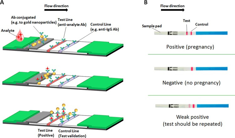
While no information is given about how the intermediate results were handled (or whether the assay itself generates more than one grades of intermediate results), it is conceivable that these were handled differently by the investigators . For example it is possible that intermediate results the manufacturer labelled as positive in their validation, were labeled as negative by the investigators. Even more likely, the participant samples were handled differently by the investigators, so that the antibody levels required to give a positive result differed in the Santa Clara study relative to the tests run by the manufacturer. In either case, the Receiver Operating Characteristic (ROC) curve in the field differs from the one of the manufacturer. Furthermore, we have very little evidence that it will not differ again in future applications. Finally, there is the possibility of good old fashioned sampling variability in the performance of the assay in the gold standard samples, without any actual substantive differences in the assay performance. Hence, the two main possibilities we considered are:
- Common Test Characteristic Model: We assume that random variation in the performance of the test in the two gold standards is at play, and we estimate a common sensitivity and specificity over the two gold standard sets. In probabilistic terms, we will assume the following model for the true positive and negative rates in the two gold standard datasets :
- and
- .
In these expressions, the TP, FN, TN, FP stand for the True Positive, False Negative, True Negative and False Positive respectively, while the subscript, i, indexes the two gold standard datasets.
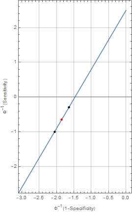
- Shifted along (the) ROC Model: In this model, we assume a bona fide shift in the characteristics of the assay when tested in the gold standard tests. This variation in characteristics, is best conceptualized as a shift along the straight line in the binormal, normal deviate plot . This plot transforms the standard ROC plots of sensitivity v.s. 1-specificity so that the familiar ROC bent curves look like straight lines. Operationally, we assume that there will be run specific variation in the assay characteristics when it is applied to future samples. The performance of the assay in the two gold standard sets provide a measure of this variability, which may resurface in subsequent use of the assay. When analyzing the data from the Santa Clara survey, we will acknowledge this variability by assuming that the assay performance (sensitivity/specificity) in this third application (red) interpolates the performance noted in the two gold standards (black).
The shift-along the ROC model is specified by fitting separate specificities and sensitivities for the two gold standard datasets, which are then transformed into the binormal plot scale , averaged and then transformed back to normal probability scale to calculate an average sensitivity and specificity. For computational reasons, we parameterize the models for the sensitivity and specificity in logit space. This parameterization also allows us to explore the sensitivity of the model to the choice of the model priors for the Bayesian analysis.
Model for the observed positive rates

The model for the observed positive counts is a binomial law , relating the positive tests in the Santa Clara sample to the total number of tests:
Priors
For the common test characteristic model, we will assume standard, uniform, non-informative priors for the Sensitivity, Specificity and Prevalence. The model may be fit with the following STAN program:
| 1234567891011121314151617181920212223242526272829303132333435363738394041424344454647484950 | functions {}data { int casesSantaClara; // Cases in Santa Claraint NSantaClara; // ppl sampled in Santa Clara int TPStanford; // true positive in Stanfordint NPosStanford; // Total number of positive cases in Stanford dataset int TNStanford; // true negative in Stanfordint NNegStanford; // Total number of negative cases in Stanford dataset int TPManufacturer; // true positive in Manufacturer datasetint NPosManufacturer; // Total number of positive cases in Manufacturer dataset int TNManufacturer; // true negative in Manufacturer datasetint NNegManufacturer; // Total number of negative cases in Manufacturer dataset }transformed data { }parameters {real<lower=0.0,upper=1.0> Sens;real<lower=0.0,upper=1.0> Spec;real<lower=0.0,upper=1.0> Prev; }transformed parameters { }model { casesSantaClara~binomial(NSantaClara,Prev*Sens+(1-Prev)*(1-Spec));TPStanford~binomial(NPosStanford,Sens);TPManufacturer~binomial(NPosManufacturer,Sens);TNStanford~binomial(NNegStanford,Spec);TNManufacturer~binomial(NNegManufacturer,Spec); Prev~uniform(0.0,1.0);Spec~uniform(0.0,1.0);Spec~uniform(0.0,1.0);}generated quantities {real totposrate;real rateratio;totposrate = (Prev*Sens+(1-Prev)*(1-Spec));rateratio = Prev/totposrate; |
For the shifted-along-ROC model, we explored two different settings of noninformative priors for the logit of sensitivity and specificity:
- a logistic(0,1) prior for the logit of the sensitivities and specificities that is mathematically equivalent to a uniform prior for the sensitivity and specificity in the probability scale.
- a normal(0,1.6) prior for the logits. While these two densities are very similar, the normal (black) has thinner tails, shrinking the probability estimates more than the logistic one (red) .

The shifted-ROC model is fit by the following STAN code (only the normal prior model is inlined below)
| 1234567891011121314151617181920212223242526272829303132333435363738394041424344454647484950515253545556575859606162636465666768 | functions {}data { int casesSantaClara; // Cases in Santa Claraint NSantaClara; // ppl sampled in Santa Clara int TPStanford; // true positive in Stanfordint NPosStanford; // Total number of positive cases in Stanford dataset int TNStanford; // true negative in Stanfordint NNegStanford; // Total number of negative cases in Stanford dataset int TPManufacturer; // true positive in Manufacturer datasetint NPosManufacturer; // Total number of positive cases in Manufacturer dataset int TNManufacturer; // true negative in Manufacturer datasetint NNegManufacturer; // Total number of negative cases in Manufacturer dataset }transformed data { }parameters {real<lower=0.0,upper=1.0> Prev;real logitSens[2];real logitSpec[2]; }transformed parameters {real<lower=0.0,upper=1.0> Sens;real<lower=0.0,upper=1.0> Spec; // Use the sensitivity and specificity by the mid point between the two kits // mid point is found in inv_Phi space of the graph relating Sensitivity to 1-Specificity// note that we break down the calculations involved in going from logit space to inv_Phi// space in the generated quantities sessions for clarity Sens=Phi(0.5*(inv_Phi(inv_logit(logitSens[1]))+inv_Phi(inv_logit(logitSens[2]))));Spec=Phi(0.5*(inv_Phi(inv_logit(logitSpec[1]))+inv_Phi(inv_logit(logitSpec[2]))));}model { casesSantaClara~binomial(NSantaClara,Prev*Sens+(1-Prev)*(1-Spec));TPStanford~binomial_logit(NPosStanford,logitSens[1]);TPManufacturer~binomial_logit(NPosManufacturer,logitSens[2]); TNStanford~binomial_logit(NNegStanford,logitSpec[1]);TNManufacturer~binomial_logit(NNegManufacturer,logitSpec[2]); logitSens~logistic(0.0,1.0); logitSpec~logistic(0.0,1.0); Prev~uniform(0.0,1.0);}generated quantities {// various post sampling estimatesreal totposrate; // Total positive ratereal kitSens[2]; // Sensitivity of the kits real kitSpec[2]; // Spec of the kitsreal rateratio; // ratio of prevalence to total positive rate totposrate = (Prev*Sens+(1-Prev)*(1-Spec));kitSens=inv_logit(logitSens);kitSpec=inv_logit(logitSpec);rateratio = Prev/totposrate;} |
Estimation of the Prevalence of COVID19 Seropositivity in Santa Clara County
Preprint author analyses and interpretation
Table 2 of the preprint summarizes the estimates of the prevalence of seropositivity in Santa Clara. This table is reproduced below for ease of reference
| Approach | Point Estimate | 95% Confidence Interval | |
| Unadjusted | 1.50 | 1.11 – 1.97 | |
| Population-adjusted | 2.81 | 2.24-4.16 | |
| Population and test performance adjusted | Manufacturer’s data | 2.49 | 1.80 – 3.17 |
| Stanford data | 4.16 | 2.58 – 5.70 | |
| Manufacturer + Stanford Data | 2.75 | 2.01 – 3.49 |
Estimated Prevalence of COVID19 Seropositivity Bendavid et al
The unadjusted estimate is computed on the basis of the observed positive counts (50/3,330 tests) and the population adjusted estimate is obtained by accounting for the non-representativeness of the sample using post-stratification weights. Finally, the last 3 rows give the estimates of the prevalence while accounting for the test characteristics. The basis of the comment that the prevalence of COVID19 infection is 50-85 fold higher is based on the estimated point prevalence of 2.49 and 4.16 respectively. Computation of these estimates, require the sensitivity and specificity for the immunoassay which the authors quote as:
Our estimates of sensitivity based on the manufacturer’s and locally tested data were 91.8% (using the lower estimate based on IgM, 95 CI 83.8-96.6%) and 67.6% (95 CI 50.2-82.0%), respectively. Similarly, our estimates of specificity are 99.5% (95 CI 98.1-99.9%) and 100% (95 CI 90.5-100%). A combination of both data sources provides us with a combined sensitivity of 80.3% (95 CI 72.1-87.0%) and a specificity of 99.5% (95 CI 98.3-99.9%).
The results obtained are crucially dependent upon the values of the sensitivity and specificity, something that the authors explicitly state in the discussion:
For example, if new estimates indicate test specificity to be less than 97.9%, our SARS-CoV-2 prevalence estimate would change from 2.8% toless than 1%, and the lower uncertainty bound of our estimate would include zero. On the other hand, lower sensitivity, which has been raised as a concern with point-of-care test kits, would imply that the population prevalence would be even higher. New information on test kit performance and population should be incorporated as more testing is done and we plan to revise our estimates accordingly.
While the authors claim they have accounted for these test characteristics, the method of adjustment is not spelled out in detail in the main text. Only by looking into the statistical appendix do we find the following disclaimer about the approximate formula used:
There is one important caveat to this formula: it only holds as long as (one minus) the specificity of the test is higher than the sample prevalence. If it is lower, all the observed positives in the sample could be due to false-positive test results, and we cannot exclude zero prevalence as a possibility. As long as the specificity is high relative to the sample prevalence, this expression allows us to recover population prevalence from sample prevalence, despite using a noisy test.
In other words, the authors are making use of an approximation, that relies on a assumption about the study results that may or may not be true. But if one is using such an approximation, then one has already decided what the results and the test characteristics should look like. We will not make such assumption in our own calculations.
Bayesian Analysis
The Bayesian analyses we report here roughly corresponds to a combination that Bendavid et al did not consider, namely an analysis using only the test characteristics, but without the post-stratification weights. Even though a Bayesian analysis that used such weights is possible, the authors do not report the number of positives and negatives in each strata, along with the relevant weights. If this information had been made available, then we could repeat the same calculations and see what we obtain. While, I can’t reproduce the exact analysis examination of Table 2 in Bendavid et al suggests that weighting should increase the prevalence by a “fudge” factor. For the purpose of this section we take the fudge factor to be equal to the ratio of the prevalence after population adjustment over the unadjusted prevalence: 2.81/1.50 ~ 1.87 .
For fitting the Bayesian analyses, I used the No U Turn Sampler implemented in STAN; Isimulated five chains, using 5,000 warm-up iterations and 1,000 post-warm samples to compute summaries. Rhat for all parameters was <1.01 for all models (R and STAN code for all analyses are provided here to ensure reproducibility).santaclaraΛήψη
Sensitivities and specificities for the three Bayesian analyses: common-parameters, shifted-along-ROC (logistic prior), shifted-along-ROC (normal prior) are shown below:
| Sensitivity | Model | Mean | Median | 95% Credible Interval |
| Common Parameters | 0.836 | 0.838 | 0.768 – 0.897 | |
| Shifted-along-ROC (logistic) | 0.811 | 0.813 | 0.733 – 0.882 | |
| Shifted-along-ROC (normal) | 0.810 | 0.813 | 0.734 – 0.878 | |
| Specificity | ||||
| Common Parameters | 0.993 | 0.994 | 0.986 – 0.998 | |
| Shifted-along-ROC (logistic) | 0.991 | 0.991 | 0.983 – 0.998 | |
| Shifted-along-ROC (normal) | 0.989 | 0.988 | 0.982 – 0.995 |
Bayesian Analysis of Assay Characteristics
The three models seem to yield similar, yet not identical estimates of the assay characteristic and one may even expect that the estimated prevalences would be somewhat similar to the analyses by the preprint authors.
The estimated prevalence by the three approaches (without application of the fudge factor) are shown below:
| Model | Mean | Median | 95% Credible Interval |
| Common Parameters | 1.03 | 1.05 | 0.16-1.88 |
| Shifted-along-ROC (logistic) | 0.81 | 0.81 | 0.50 – 1.84 |
| Shifted-along-ROC (normal) | 0.56 | 0.50 | 0.02 – 1.46 |
Model Estimated Prevalence (%)
Application of the fudge factors would increase the point estimates to 1.93%, 1.52% and 1.05% which more than 50% smaller than the prevalence estimates computed by Bendavid et al. To conclude our Bayesian analyses, we compared the marginal likelihoods of the three models by means of the bridge sampler. This computation allows us to roughly see which of the three model/prior combinations is supported by the data. This analysis provided overwhelming support for the Shifted-along-ROC model with the normal (shrinkage) prior:
| Model | Posterior Probability |
| Common Parameters | 0.032 |
| Shifted-along-ROC (logistic) | 0.030 |
| Shifted-along-ROC (normal) | 0.938 |
Conclusions
In this rather long post, I undertook a Bayesian analysis of the seroprevalence survey in Santa Clara county. Contrary to the author’s assertions, this formal Bayesian analysis suggests a much lower seroprevalence of COVID19 infections. The estimated fold increase is only 20 times higher (point estimate), rather than 50-80 fold higher and with a 95% credible interval 0.75 -55 fold for the most probable model.
The major driver of the prevalence, is the specificity of the assay (not the sensitivity), so that particular choices for this parameter will have a huge impact on the estimated prevalence of COVID19 infection based on seroprevalence data. Whereas the common parameter and the shifted-along-ROC models yield similar estimates for the same prior (the uniform in probability scale is equivalent to standard logistic in the logit scale), a minor change to the priors used by the shifted-along-ROC model, leads to results that are qualitatively and quantitatively different. The sensitivitity of the estimated prevalence to the prior, suggests that the assay performance data are not sufficient to determine either the sensitivity or the specificity with precision. Even the minor shrinkage implied by changing the prior from the standard logistic to the standard normal , provides a small, yet crucial protection against overfitting and leads to a model with extremely sharp marginal posterior likelihood.
Are the Bayesian analysis results reasonable? I still can’t trust the quality and the biases inherent in the source data, but at least the calculations were done lege artis . Interestingly enough, the estimated prevalence of COVID19 infection (1-2%) by the Bayesian methodology described here, is rather similar to the prevalence (<2%) reported in Telluride, Colorado.
The analysis reported herein could be made a lot more comparable to the analyses reported by Bendavid et al, if the authors had provided the strata data (positive and negative test results and sample weights). In the absence of this information, the use of fudge factors is the best equivalent approximation to the analyses reported in the preprint.
Is the Santa Clara study useful for our understanding of the COVID19 epidemic?
I feel that the seroprevalence study in Santa Clara is not the “bombshell” study that I initially felt it would be (so apologies to all my Twitter followers whom I may have misled). There are many methodological issues starting with the study design and extending to the author’s analyses of test performance. Having spent hours troubleshooting the code (and writing the blog post!), my feelings align perfectly with Andrew Gelman’s:
I think the authors of the above-linked paper owe us all an apology. We wasted time and effort discussing this paper whose main selling point was some numbers that were essentially the product of a statistical error.
I’m serious about the apology. Everyone makes mistakes. I don’t think they authors need to apologize just because they screwed up. I think they need to apologize because these were avoidable screw-ups. They’re the kind of screw-ups that happen if you want to leap out with an exciting finding and you don’t look too carefully at what you might have done wrong.
COVID19 is a serious disease, which is far worse than the flu in terms of contagiousness, severity and lethality of the severe forms and level of medical intensive care support needed to avert a lethal outcome. Knowing the prevalence will provide one of the many missing pieces of the puzzle we are asked to solve. This piece of information will allow us to mount an effective public health response and reopen our society and economy without risking countless lives.
Disclaimer: I provided the data for my analyses with the hope that someone can correct if I am wrong and corroborate me if I am right. Open Science is the best defense against Bad science and making the code available is a key step in the process.
Christos Argyropoulos is a clinical nephrologist, amateur statistician and Division Chief of Nephrology at the University of New Mexico Health Sciences Center. This post originally appeared on his blog here.
